Welcome to DU!
The truly grassroots left-of-center political community where regular people, not algorithms, drive the discussions and set the standards.
Join the community:
Create a free account
Support DU (and get rid of ads!):
Become a Star Member
Latest Breaking News
General Discussion
The DU Lounge
All Forums
Issue Forums
Culture Forums
Alliance Forums
Region Forums
Support Forums
Help & Search
Science
Related: About this forumThe amplitude and origin of sea-level variability during the Pliocene epoch
The paper I'll discuss in this post is this one: The amplitude and origin of sea-level variability during the Pliocene epoch (Grant et al, Nature volume 574, page s237–241 (2019).
This past Thursday I posted a similar paper about this epoch, which was also published in Nature, in the same issue, just above this one.
During the Pliocene Epoch, which was from 3 to 5 million years ago, the concentration of carbon dioxide in the atmosphere apparently surged (for a few hundred thousand years) to around 450 ppm, which, since we are doing nothing meaningful about climate change, we will hit in about 15 to 20 years.
The authors here use a different approach than the approach I discussed on Thursday.
From the abstract:
Earth is heading towards a climate that last existed more than three million years ago (Ma) during the ‘mid-Pliocene warm period’1, when atmospheric carbon dioxide concentrations were about 400 parts per million, global sea level oscillated in response to orbital forcing2,3 and peak global-mean sea level (GMSL) may have reached about 20 metres above the present-day value4,5. For sea-level rise of this magnitude, extensive retreat or collapse of the Greenland, West Antarctic and marine-based sectors of the East Antarctic ice sheets is required. Yet the relative amplitude of sea-level variations within glacial–interglacial cycles remains poorly constrained. To address this, we calibrate a theoretical relationship between modern sediment transport by waves and water depth, and then apply the technique to grain size in a continuous 800-metre-thick Pliocene sequence of shallow-marine sediments from Whanganui Basin, New Zealand. Water-depth variations obtained in this way, after corrections for tectonic subsidence, yield cyclic relative sea-level (RSL) variations. Here we show that sea level varied on average by 13 ± 5 metres over glacial–interglacial cycles during the middle-to-late Pliocene (about 3.3–2.5 Ma). The resulting record is independent of the global ice volume proxy3 (as derived from the deep-ocean oxygen isotope record) and sea-level cycles are in phase with 20-thousand-year (kyr) periodic changes in insolation over Antarctica, paced by eccentricity-modulated orbital precession6 between 3.3 and 2.7 Ma. Thereafter, sea-level fluctuations are paced by the 41-kyr period of cycles in Earth’s axial tilt as ice sheets stabilize on Antarctica and intensify in the Northern Hemisphere3,6.
The authors review, as the authors described in my previous post, the techniques for evaluating the sea level in the geological past:
Pliocene sea-level changes have been reconstructed using a variety of geological techniques including: (i) marine benthic oxygen-isotope (?18O) records paired with Mg/Ca palaeothermometry (a proxy for global ice volume)4, (ii) an algorithm incorporating sill-depth, salinity and the ?18O record from the Mediterranean and Red seas8, (iii) uplifted palaeo-shorelines4,9, and (iv) backstripped continental margins2,4.
...and describe some significant limitations, for example with the ?18O method...
Although the global benthic ?18O stack provides one of the most detailed proxies for orbital-scale (glacial–interglacial) climate variability during the Pliocene3, the signal comprises both ocean-temperature and ice-volume effects that are not easily deconvolved2,4,11. Moreover, calibrations of ?18O to sea level do not account for the nonlinear relationship between marine-based ice-volume change and the ?18O of sea water12.
They then describe their approach:
Our record, which we term PlioSeaNZ, is constructed from sedimentary cycles that represent fluctuations between middle- to outer-shelf water depths that were recovered in sediment cores (3.3–3.0 Ma) and outcrop sections exposed in the Rangitikei River valley (2.9–2.5 Ma). Sediments accumulated continuously at rates of >1 m kyr?1 (see Methods). Erosion during lowstands did not occur on the middle to outer shelf, because the changes in the amplitude of Pliocene RSL were accommodated in these environments without experiencing wave base erosion or subaerial exposure. The palaeo-environmental interpretation of the cores and outcrops is described in detail in ref. 6 and summarized in Supplementary Figs. 1 and 2.
Reference 6 is this one, from the same group:
Mid- to late Pliocene (3.3–2.6 Ma) global sea-level fluctuations recorded on a continental shelf transect, Whanganui Basin, New Zealand (Grant et al Quaternary Science Reviews Volume 201, 1 December 2018, Pages 241-260) I have not personally accessed this paper.
A few more details on their approach:
We have developed a novel approach that utilizes the well-established relationship between sediment grain size and water depth14 to calculate palaeo-water-depth changes. Wave energy produces a decreasing near-bed velocity at increasing water depths across the shelf, resulting in a seaward-fining sediment profile14. Modern observations support theoretical calculations that show that maximum water depth for a given grain size corresponds to the depth at which wave-induced near-bed velocity exceeds the critical velocity required for sediment transport14 (see Methods; Extended Data Fig. 1a). Thus, the percentage of sand (grains of size 63–2,000 µm) in closely spaced geological samples can be used to estimate changes in palaeo-water depth provided that the sediment is wave-graded6 and that Pliocene wave climate can be broadly estimated.
Some pictures from the text:
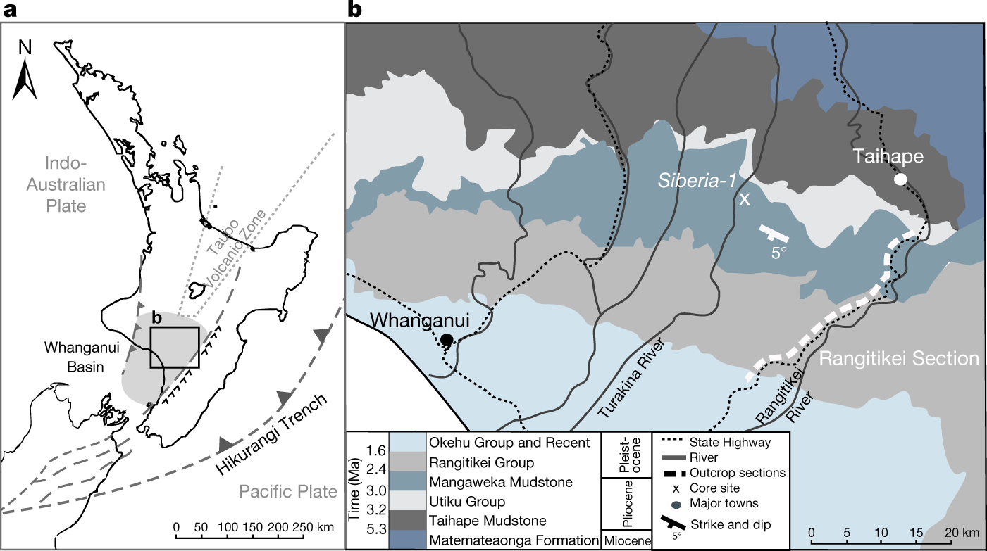
The caption:
a, Overview of North Island. Whanganui Basin (grey shaded region) formed behind the Hikurangi subduction zone as part of a southward-migrating pattern of lithospheric flexure associated with southwestward propagation of the subducting Pacific Plate beneath the Indo-Australian Plate2. b, Magnified view of boxed area in a. Subsequent uplift in central North Island during the last 1 Ma, in response to redistribution of lithosphere over the mantle2, has exposed Plio-Pleistocene, shallow-marine sediments onshore where they tilt southwestward at 5°. Locations of Siberia-1 drill site (white ‘x’ marker) and Rangitikei River outcrop (bold dashed white line) are shown. Geological data in b adapted from GNS Science.
 ?as=webp
The caption:
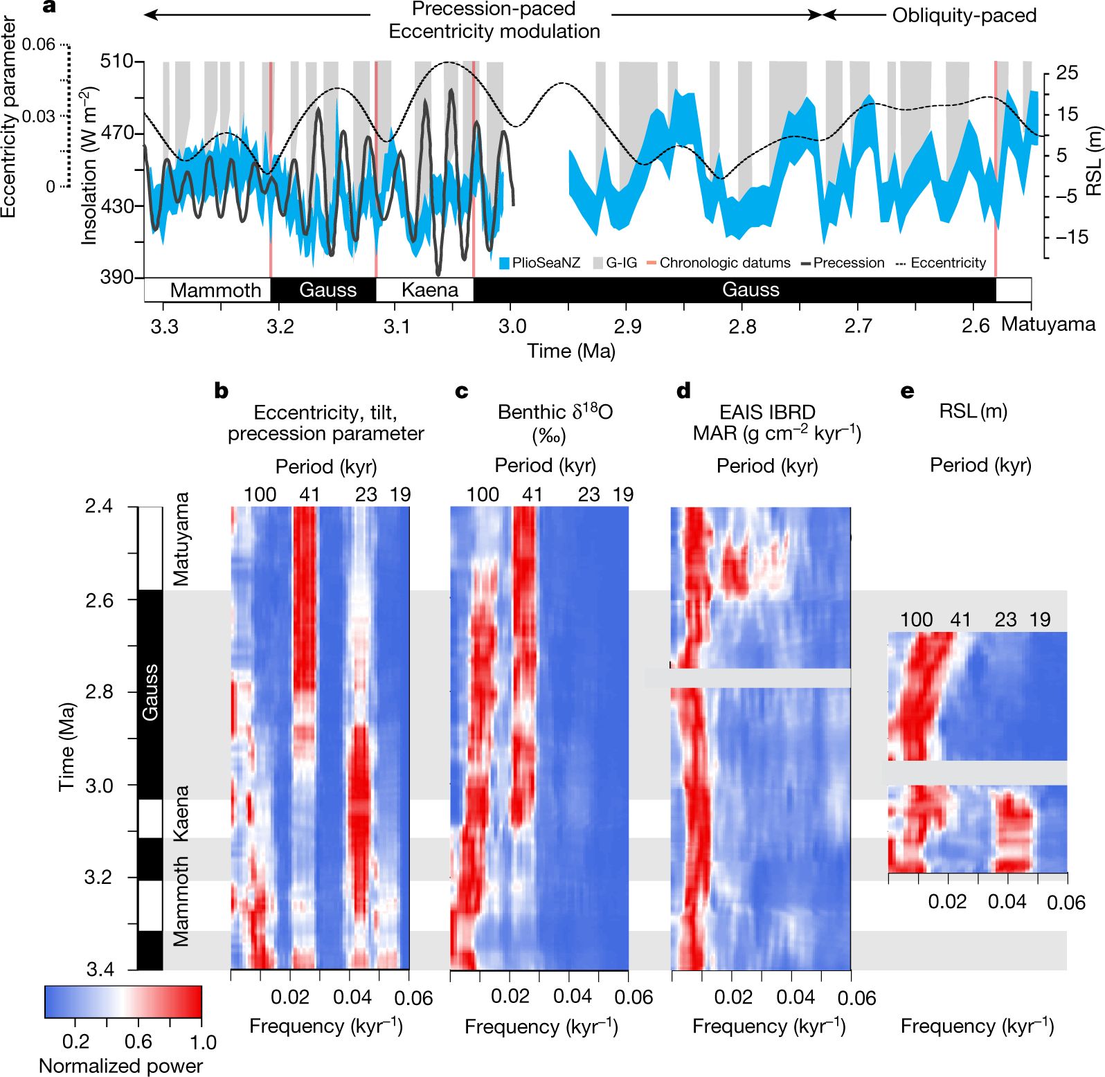
a, PlioSeaNZ RSL record (right-hand vertical axis), unregistered to the present day, for the middle to late Pliocene, with uncertainty represented by the shaded blue band, which does not exceed ±5.6 m (see Methods). Glacial–interglacial (G–IG) transitions are marked by the shaded grey bands. The age model is untuned and derived from linear sedimentation rates between magnetic reversals (orange-pink lines) with an uncertainty of ±5 kyr. Summer insolation (1 January) at 65° S (black curve) and the eccentricity parameters (dashed curve) are shown for ref. 18 (left-hand vertical axes). b–e, Multi-taper method time–frequency analyses (see Methods) displaying normalized power (colour scale) for eccentricity, obliquity and precession insolation parameter18 (b), the global benthic foraminifera ?18O stack3 (c), EAIS IBRD mass accumulation rate21 (d) and our RSL record (e; PlioSeaNZ Whanganui Basin). Periods are denoted for eccentricity (100 kyr), obliquity (41 kyr) and precession (23 and 19 kyr).
The caption:
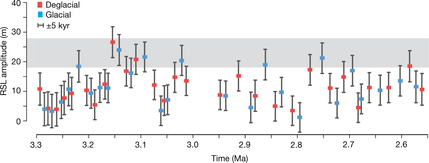
Amplitudes of deglacial (glacial–interglacial; pink squares; n = 28) and glacial (interglacial–glacial; blue squares; n = 26) RSL changes are shown with error bars representing ±1 s.d. (after equation (10)) with an average of 5.1 m, and age uncertainty is ±5 kyr (as discussed in the text, and shown in the figure key). The grey shaded band (about 23 ± 5 m) shows the possible contribution from the marine-based sectors of the AIS (about 23 m)28 and the GIS estimated as19 ±5 m depending on the interhemispheric phase relationship. Glacial–interglacial amplitudes higher than approximately 28 m exceed the ice inventory of the marine-based AIS sectors (22.7 m; ref. 28) and the GIS (5 m; ref. 19) based on present-day volumes.
https://www.nature.com/articles/s41586-019-1619-z/figures/4
The caption:
Modelled result of 10 kyr linear melting between glacial and interglacial states required for 20 m of equivalent ESL, and according to the reference mantle viscosity profile30. a, 20 m ESL released from AIS only. b, AIS and GIS synchronously release 15 m and 5 m ESL, respectively. c, AIS releases 25 m ESL while GIS accumulates 5 m ESL (that is, in anti-phase). d, AIS and NHIS synchronously release 10 m ESL. The white band represents ±0.05 of the eustatic mean (bold black line), which equates to ±1 m. The Whanganui site is highlighted by the red and white bullseye on New Zealand.
AIS is the antarctic ice sheet, GIS, greenland ice sheet.
They speak on the effect of rotational precession changes the insolation patterns drive this historical warming, and that this in turn, they argue, means that the Antarctic Ice Sheet is more prominent in driving sea level rises.
This does not mean that they exclude carbon dioxide, far from it.
From their conclusion:
In conclusion, our results provide new constraints on polar ice-sheet and global sea-level variability during the middle and late Pliocene, that are: (i) independent of estimates from the global benthic ?18O stack3 and other geochemical proxies4, and (ii) broadly consistent with AIS models7,19,20 that simulate a contribution of 13–17 m to global sea-level rise above present. Because our record cannot be registered to present-day sea level, we cannot directly constrain the magnitude of peak Pliocene GMSL above present. Regardless, our results provide key insights into AIS sensitivity when Earth’s climate equilibrates at a CO2 partial pressure of about 400 ppm. Furthermore, if all the variability in the PlioSeaNZ record was above present-day sea level, then GMSL during the warmest mid-Pliocene interglacial was no more than +25 m. Although ice-sheet, ocean and continental geometries were subtly different during the mid-Pliocene, our results suggest that major loss of Antarctica’s marine-based ice sheets, and an associated GMSL rise of up to 23 m, is likely if CO2 partial pressures remain above 400 ppm.
Have a pleasant Sunday afternoon.
InfoView thread info, including edit history
TrashPut this thread in your Trash Can (My DU » Trash Can)
BookmarkAdd this thread to your Bookmarks (My DU » Bookmarks)
0 replies, 873 views
ShareGet links to this post and/or share on social media
AlertAlert this post for a rule violation
PowersThere are no powers you can use on this post
EditCannot edit other people's posts
ReplyReply to this post
EditCannot edit other people's posts
Rec (3)
ReplyReply to this post